Marginal Utility Analysis

What is marginal utility analysis?

Utility is the pleasure, satisfaction, joy or happiness that a consumer derives from using a good or service. Marginal utility analysis is one of the approaches to studying utility in economics. It is based on the ability to measure utility in quantitative units, called utils. It is also called the cardinalists’ approach.

Content

Total utility and marginal utility

As a consumer increases the quantity of a product he or she consumes, the sum of the satisfaction he obtains from all the units consumed increases. The combined satisfaction from the consumption of all the units of a product is total utility while the satisfaction derived from an extra unit of a product is marginal utility.

The marginal utility curve slopes downward from left to right because the utility derived from each additional unit of the product consumed declines ( see marginal utility in Figure 1 below). The total utility increases first; then it reaches a maximum point before declining (Figure 1 below). Continuous consumption of more units of a product makes the consumer attain the point of satiety or maximum satisfaction (see point A in Figure 1). If he or she still goes on using more and more units of the product, the total utility will start to decrease because the amount of satisfaction from each extra unit added to the total utility keeps declining.

How to calculate marginal utility

Marginal utility is the change in total utility due to the consumption of an additional unit of a good.

MU = Change in total utility ÷ Change in quantity

Table 1: Computation of marginal utility

Quantity of oranges	Total Utility (TU)	Marginal Utility (MU)
0	0	–
1	15	15
2	25	10
3	25	0
4	22	-3
5	14	-8

Calculation of Marginal Utility (MU):

MU = Change in total utility ÷ Change in quantity

For 1, MU = 15-0/1-0 = 15 For 2, MU = 25-15/2-1 = 10
For 3, MU = 25-25/3-2 = 0 For 4, MU = 22-25/4-3 = -3
For 5, MU = 14-22/5-4 = -8

Relationship between total utility and marginal utility

Initially, the combined satisfaction (total utility in Figure 1 below) rises as more units are being consumed. But the increase is at a decreasing rate owing to a continuously declining marginal utility. When the point of satiety (Point A) is reached, the total utility is at its peak while the marginal utility is zero.

From Table 1 above, the consumer reaches point of satiety when 3 units of the product have been consumed. Any additional consumption after this will lead to a decrease in total utility because every extra unit consumed will now have a negative utility. That is to say, negative utility is added from this point to total utility so the overall satisfaction keeps diminishing. For example, in Table 1 above, the consumption of the 4th unit gives a marginal utility of -3 and the total utility fell to 22 (25-3). A negative marginal utility means that the product is no longer useful to the consumer; he or she is experiencing disutility or dissatisfaction.

Figure 1: Marginal and total utility curves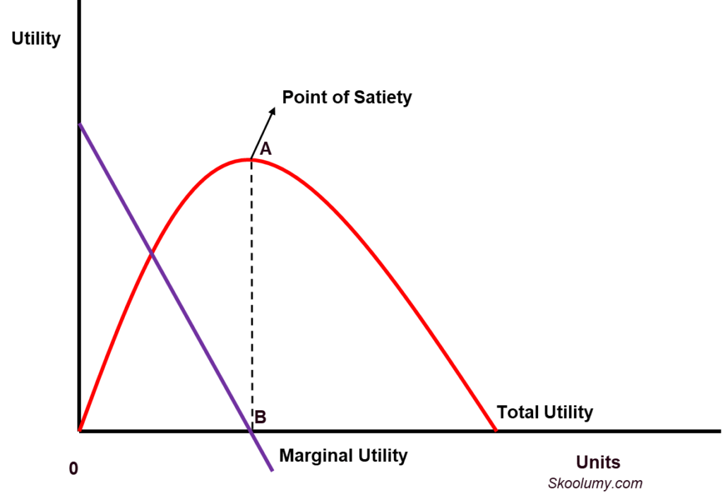

The law of diminishing marginal utility

The law says “as more and more quantity of a particular product are consumed, the satisfaction derived from every additional unit keeps on falling”. The idea was first conceived by Gossen Hermann Heinrich, hence it is sometimes called Gossen’s First Law. Alfred Marshall improved Gossen’s idea and made it a law. From Table 1 above, the 1st unit adds 15 utils to total utility, the 2nd unit adds 10, the 3rd unit adds 0, etc.

The law holds only when certain conditions are met. In other words, there are limitations to the law of diminishing marginal utility because the law was made under certain assumptions. They include:

Measurable utility

Utility must be capable of being measured. In reality, utility is psychological and cannot be measured accurately. The amount of satisfaction attributable to a particular product differs from time to time and from person to person. It all depends on the mental state of the user at the point in time.

The units must be indistinguishable

The units must be of the same kind or nature such that they are not perceived as different by the consumer. All the units of the product must be identical in magnitude, taste and colour.

No discontinuity in consumption

There must not be a break in consumption; all the units have to be consumed at the same time. There is a possibility for the satisfaction to increase if the consumer consumes a unit now and consumes additional units later.

Tastes, incomes and preferences are constant

The tastes, incomes, habits and preferences of consumers must remain unchanged. A change in any of these may lead to a rise in satisfaction as more and more units are consumed.

Rational consumer

Economic theory, generally, assumes that the consumer is a rational being who obtains maximum satisfaction from the good he uses. Many factors make the consumer irrational, such as the inability to get accurate information on the usefulness of the product and social influence. An irrational person may be addicted to a product and utility continues to increase as he buys more units of the product.

The product must be divisible

The law does not apply to products that are not divisible, like a car. The consumer cannot quantify his utility at a point in time because the benefit spans months or years. Again, the consumer cannot split the product into smaller units to determine the satisfaction from consuming additional units.

Prices must be constant

The prices of the product and its substitutes must be unchanged. If the price of the product increases relative to the substitute, the consumer may not want to buy additional units of the product; rather, he will switch to the cheaper substitute.

The usefulness of the law of diminishing marginal utility

Usefulness to producers and marketers

Producers realise that as consumers continue to use their products, their satisfaction or interest will decrease at a certain point. So, they try from time to time to improve the product quality, features, design, colour and packaging in order to sustain consumers’ interest. Consumers perceive the product as new when there is product innovation.

Usefulness to the government

The satisfaction one obtains from obtaining more money declines after a certain point. A wealthy person does not have increased happiness from getting additional money, but a poor man derives increasing satisfaction each time he makes more money. That is why the government takes more taxes from the rich than the poor, using progressive taxation. Progressive taxation is one in which the tax rate increases as income increases.

Explains the law of demand better

It is the basis on which the law of demand is formed. Why is the price high when the quantity decreases and low when the quantity increases? Firstly, you must realise that the price a consumer is willing to pay for a product is determined by the amount of satisfaction or utility derived from its consumption. The marginal utility decreases as the consumer consumes increasing units of the product. Thus, he will be willing to pay a lower price as the quantity increases. But he will attach a higher price if the quantity consumed is low because the marginal utility remains high.

Explains the paradox of value

The law explains why an essential good has a low price while a high price is often attached to a non-essential good. Marginal utility and price decrease with the increasing quantity or supply of a product. Water, for example, is more beneficial than gold. However, the price of water is far less than the price of gold. This is because water is available in great quantity, which makes its marginal utility low and price low. Gold is scarce; every extra unit of gold obtained has more utility and attracts a higher price.

Consumer equilibrium and the law of equi-marginal utility

A rational man seeks to maximise his total utility or satisfaction from his consumption. He achieves equilibrium only when he spends his money in a way that will maximise the satisfaction he derives from the products bought. There are two approaches used to determine consumer equilibrium, namely marginal utility analysis and indifference curve analysis. The marginal utility analysis is based on the assumption that utility can be measured; it is also called cardinal utility analysis. The other method, indifference curve analysis, is on the premise that utility cannot be measured. Indifference curve analysis is also called ordinal utility analysis.

The law of equi-marginal utility is a way of determining consumer equilibrium in marginal utility analysis. The law says “the consumer can only attain equilibrium when the marginal utility per price is the same for all the products he purchases with his income”. In other words, the marginal valuations of all the goods consumed are the same at equilibrium. The other names for the law include equi-marginal principle, the law of maximum satisfaction, the law of substitution and Gossen’s second law.

The equi-marginal principle formula is given as:

MU_a = MU_b
P_a P_b

It is subject to income limitation which is stated as:
P_aQ_a + P_bQ_b

Where

MU_a = Marginal utility of good a
MU_b = Marginal utility of good b
P_a = Price of good a
P_b = Price of good b
Q_a = Quantity of good a
Q_b = Quantity of good b

If MU_a/P_a is greater than MU_b/P_b, he has to buy more of good a and less of good b since the satisfaction from good a is greater. He/she continues to buy more of good a until the equilibrium is restored due to the law of diminishing marginal utility. If MU_a/P_ais less than MU_b/P_b, the consumer can maximise his utility by buying less of good a and more of good b which has higher utility. Buying more of good b will reduce its marginal utility until the equilibrium condition is reestablished.

The law of equi-marginal utility is based on some assumptions which include:

1. This is cardinal utility analysis and it is believed that utility can be measured. Utility is measured in utils and marginal utility is calculated from the given total utility.

2. The law only works when dealing with a rational consumer who seeks to maximise his/her utility from the goods he consumes.

3. The consumer’s income must be known because the money he/she has is constraint to the quantities of goods he/she can buy. The total expenditure of the consumer must be equal to the amount of his/her income.

4. The prices of the goods involved must be known. This makes it possible to determine the marginal valuation of each product by dividing marginal utility by the price.

5. The law of diminishing marginal utility must be applicable. Given a consumption bundle, the only way to maximise utility is to buy more of the product with higher satisfaction at the expense of the one that gives fewer utils. The marginal utility will decrease when a consumer continues purchasing more quantity of a particular product until the marginal valuations of all products consumed are equal.

6. Money can be used to determine the amount of utility derived from a product. It is assumed that the utility from each extra unit of money a consumer obtains is unchanged. The marginal utility of extra money will decrease if one is already rich.

Worked example on the law of equimarginal utility

Table 2 below is a schedule of the total utility of a consumer from two products, Product X and Product Y. The price of Product X is $10 while the price of Product Y is $5. He has a total income of $40. What quantity of both goods will he buy if he is to be in equilibrium?

Table 2: Schedule showing the total utility from consuming Product X and Product Y

Quantity of X	Total Utility of X	Quantity of Y	Total Utility of Y
1	100	1	50
2	125	2	60
3	145	3	68
4	155	4	73
5	160	5	76

The steps involved are:
1. Calculate the marginal utility, MU/Price for both products (see Table 3 and Table 4 below).

2. Identify the quantity of both goods where their MU/Price are equal, i.e., 3 units of Product X and 2 units of Product Y.

3. Compute the total expenditure on the quantities of both goods that maximise utility. The total expenditure should be equal to the consumer’s income, i.e., 3($10) + 2($5) = $40. The consumer is in equilibrium when he buys 3 units of Product X and 2 units of Product Y.

Table 3: Computation of marginal valuation of product X

Quantity of X	Total Utility of X	Marginal Utility of X	MUX/PX
1	100	–	–
2	125	25	2.5
3	145	20	2*
4	155	10	1
5	160	5	0.5

Table 4: Computation of marginal valuation of Product Y

Quantity of Y	Total Utility of Y	Marginal Utility of Y	MUY/PY
1	50	–	–
2	60	10	2*
3	68	8	1.6
4	75	7	1.4
5	78	3	0.6

Derivation of the demand curve from marginal utility

The price paid by the consumer is determined by the amount of satisfaction obtained from each extra unit of the product purchased. He will be willing to pay a low price if the marginal utility per pound (or dollar) is low and a high price for high marginal utility per pound (or dollar). And the more the units of a product he/she consumes, the less the utility from every additional unit. Consequently, the price keeps getting smaller as the amount consumed increases. The consumer values the product more and attaches a high price if he has less of it. This explains the law of demand which says the higher the quantity the lower the price and the lower the quantity the higher the price. Consequently, the demand curve slopes downwards.

Equi-marginal principle and the demand curve

The equi-marginal principle is stated as:

MU_a = MU_b
P_a P_b

Rational consumers will buy more units of a product when the marginal utility per price rises; they will buy fewer units if the marginal utility per price falls. If the price of Good a rises, MU_a/P_a falls, causing a decrease in the quantity of Good a purchased. This is why a rise in price leads to a fall in the quantity demanded. If the price of Good a falls, MU_a/P_a will increase, thereby leading to a rise in the quantity bought. This explains why quantity rises as price falls. Therefore, there is an inverse relationship between price and quantity demanded – the demand curve slopes downward.