Equilibrium wage rate in a perfectly competitive labour market
A perfectly competitive labour market is a type of labour market in which there are many employers who pay the same wage rate to numerous workers. Workers in this market are assumed to have identical skills. Besides, all available job opportunities and the prevailing wage rate are known to the workers who are occupationally and geographically mobile to take advantage of these opportunities. Neither the employers nor the employees have the power to alter the prevailing wage rate in their favour. In other words, no worker can successfully bargain for a wage rate above the equilibrium wage rate because there are many workers who are willing to accept the existing wage rate. Also, no employer can succeed at paying a lower wage rate than the ruling wage rate since there are numerous firms willing to pay the wage rate prevalent in the market.
Figure 1: Wage rate determination in a perfectly competitive labour market

The firm will continue to employ as long as the Marginal Revenue Product (MRP) is equal to the Marginal Factor Cost (MFC). In other words, the equilibrium wage rate is determined where MRP = MFC (We in Figure 1 above). The quantity employed is Qe. The MRP is the extra revenue brought in by the additional worker while MFC is the price paid to each extra worker. The MRP curve slopes downward since the revenue from each additional worker decreases as more and more workers are hired. This is in line with the fact that the output obtained from every additional worker declines as the number of workers employed increases. So the revenue paid to each extra worker should drop as his contribution to total output declines. The wage rate is the same for every additional worker hired; therefore, the MFC curve, which is the same as the supply curve of labour, is horizontal.
Figure 2: Industry wage rate determination in a perfectly competitive labour market

The industry faces a downward-sloping demand curve and an upward-sloping supply curve. The firms, which are many, are so small that they cannot change the shape of the industry demand curve by their individual actions. The equilibrium wage rate for the industry is determined where industry demand for labour and industry supply of labour are equal. WL is the industry equilibrium wage rate while QL is the quantity of labour hired in the industry (see Figure 2 above).
Equilibrium wage rate in an imperfect labour market
In fact, the assumptions of the perfectly competitive labour market are unrealistic. A firm may be the dominant buyer of labour in the market; this is referred to as monopsony. The firm, as a result, has a substantial influence on the wage rate paid to labour. This contradicts the assumption that the firms are wage takers that lack the power to change the wage rate. Employers may also face a trade union that collectively bargains for a group of workers, thereby acting like one seller of labour with considerable ability to negotiate a higher wage rate for its members. Furthermore, it is not possible for all the workers to have the same skills as experiences, education and training differ.
Monopsony
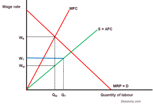
The monopsonist will continue to employ a particular number of workers as long as the MRP and MFC are equal. It employs QM workers from Figure 3 below. However, he pays a lower wage rate of WM as opposed to WR which is obtained from where MRP is equal to MFC as it can influence the wage rate being the only employer of labour. Note that WM is traced to the firm’s supply of labour curve.
Figure 3: Wage rate determination in monopsony

If the monopsonist employs an additional worker for a higher wage rate than it is currently paying the other workers, it has to pay all the workers the new rate. The cost of employing the additional worker is the sum of the wage rate paid to the new worker and the extra cost incurred to bring the rate paid to the old workers to the new level. For example, a monopsony firm employs five workers at $4 per hour. It intends to employ the sixth worker at $6 per hour. The cost of employing the sixth worker is $16; this is the sum of $6 to be paid to the sixth worker and $10 to be paid to the old workers to ensure they also get the new rate ($2 times 5).
Trade union
One of the imperfections in the labour market occurs when the firm faces a monopoly seller of labour in the form of a trade union. The union represents all the workers and collectively negotiates wage increases and better working conditions with the employer. A trade union may pressurise employers to raise the wage rate to WT (see Figure 4 below) from the wage rate of WM. QT workers will be employed by the firm as a result of the trade union negotiation. Every additional worker has to be paid WT.
Figure 4: Trade union in monopsony
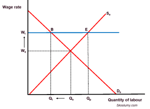
Trade unions tend to be less successful in a perfectly competitive labour market. The wage rate rises from We to Wt as a result of the activities of the union (Figure 5 below). The number of workers employed falls from Qe to Qt because higher wages increase the labour cost in the market. In Figure 4 above, the quantity of labour hired in a monopsony rose from QM to QT when a wage rate of WT is negotiated by the trade union.
Figure 5: Trade union in a perfectly competitive labour market
Minimum wage
A minimum wage is the lowest wage that can be paid to workers. The government intervenes in the labour market by promulgating a minimum wage legislation to protect the low-paid workers in the country. In a perfectly competitive market, the minimum wage has to be above the equilibrium wage rate to be effective. It will increase wages paid to workers but reduce the number of workers hired by firms since it adds to their costs. It, therefore, increases unemployment since the supply of labour will exceed the demand for labour. This is because the higher wage increases the supply of labour and reduces demand for labour. In Figure 6 below, the minimum wage rate of Wm leads to Qm workers being employed. The number of people unemployed due to the introduction of minimum wage is from C to D. Therefore, the introduction of minimum wage in a perfectly competitive labour market reduced the level of employment.
Figure 6: Minimum wage in a perfectly competitive labour market

However, a firm may bear the cost of increasing the wage rate without reducing the number of workers if the workers have special skills and are difficult to replace. The firm may also not cut down on its workforce if the wage raise increases workers’ productivity or the demand for the underlying product is high.
The introduction of a minimum wage in a monopsony labour market is more effective than in a competitive market because it is capable of increasing the wage rate and the number of workers employed at the same time. In Figure 7 below, the minimum wage of WM leads to an increase in the number of workers employed from Q1 to QM.
Figure 7: Minimum wage in a monopsony labour market

If demand for the underlying product is low or the labour cost is so high that it may lead to the closure of the business, the monoposony firm would reduce its demand for labour. In addition, if cheap capital can replace workers, the business would lay off some workers due to the introduction of a minimum wage. Capital-intensive industry would rather employ more capital instead of employing workers when a minimum wage is introduced. Therefore, the introduction of a minimum wage may not increase the employment level.